Outline
In this Kühne Impact Series, we substantiate our claim that international trade should play a central role in the fight against climate change. The key message is that “buying green” does not necessarily mean “buying local” and that a smart combination of local and foreign sourcing yields the best results. To this end, we construct an exhaustive database on the greenhouse gas emissions related to international trade flows from and to the European Union. Our first main result is that 28% of European trade flows are already green in the sense of bringing about a net reduction in greenhouse gas emissions relative to domestic sourcing. Our second main result is that a simple green sourcing rule could reduce trade-related emissions by 35%. Hence, there is a substantial green sourcing potential remaining in European trade
At the Kühne Center for Sustainable Trade and Logistics, we believe that the world should embrace international trade in the fight against climate change. The reason is that “buying green” does not necessarily mean “buying local”, because transport emissions only account for a small share of total emissions and there is large variation in production emissions across countries. Buying green – or green sourcing – instead involves comparing the production and transport emissions associated with all available sourcing options and choosing the one that minimizes the sum of both.
In this Kühne Impact Series, we substantiate this view by providing our most systematic analysis of green sourcing to date. Our analysis has three parts:
First, we construct an exhaustive database on the greenhouse gas emissions related to the international trade flows of the EU. While this database is mainly an input into the analyses discussed in the subsequent sections, it also reveals some basic information that is interesting in its own right. In particular, we find that transport emissions only account for 16% of total emissions and are less strongly related to distance than one might think.
Second, we use this database to take stock of European trade as it is. In particular, we compare the total emissions associated with each trade flow with the hypothetical alternative of “buying local”. Our main result is that 28% of European trade flows are already green in the sense of bringing about a net reduction in total emissions. However, this average masks huge variation across origins, destinations, and sectors, which we also discuss.
Third, we turn to exploring European trade as it could be. In particular, we develop a simple green sourcing rule based on a new sector-level metric that we call “foreign green sourcing potential”. A high potential simply means that transport emissions tend to be relatively low and production emissions tend to be relatively dispersed in a sector so that there is a high chance of foreign sourcing being the green choice. Our main result is that this simple green sourcing rule could reduce trade-related emissions by 35% – more than twice of what could be achieved by only “buying local”. Hence, there is a substantial green sourcing potential remaining in European trade.
Measuring trade emissions
In this section, we describe the construction of our new database. Readers who are mainly interested in our results can skip forward to the next section.
Our database records the production and transport emissions associated with the international trade in goods and services between 28 EU countries and 67 trading partners (including a residual “Rest of the World”) during the years 2003–2018.
We construct this database by estimating transport emissions and combining our estimates with pre-existing information on production emissions. We estimate transport emissions using a top-down approach building on Cristea et al (2013).1 This approach relies on data on quantities (rather than values) internationally traded and broken down by the broad modes of transport used. Combined with information on distances between countries and measures of average greenhouse gas emissions per ton-km for individual modes of transport, it is possible to estimate the CO2eq emissions associated with the transport of internationally traded goods and services.
Concretely, we combine publicly available data on production emissions for a set of 67 countries and 30 (traded) sectors from the OECD2 with trade statistics from Eurostat and IPCC technical coefficients to construct total trade-related emissions. Eurostat provides traded values and weights between the 28 EU members and the rest of the world at the CN8 product level,3 broken down by seven modes of transport: sea, air, road, rail, pipeline, self-propulsion and other, between 2001 and 2018. Where necessary, we impute the modal split of trade flows based on the geography of the origin and destination countries, the type of good transported, and the total value and weight traded. A technical appendix with the precise procedure of the data construction is available upon request. We obtain average emissions per ton-km per mode of transport from the Fifth Assessment Report of the IPCC.4 As these coefficients are provided as a range (lower and upper bound) we are in fact able to construct transport emissions under a HIGH emissions scenario (using the upper bound) or a LOW emissions scenario. We will mostly focus on the low scenario in what follows.5
We close this section by recording two basic points about transport emissions that emerge from our database and provide some helpful context to our subsequent analysis.
First, transport emissions account on average for 16% of total emissions. The production of a traded good emits on average 326 g of CO2 per dollar produced, with tremendous heterogeneity across countries, goods, and over time.6 In comparison, the transport of a good emits on average between 150 and 240 g of CO2 per dollar transported (under the LOW or HIGH scenario, respectively), with even larger variation. When accounting for these two types of emissions in trade, we find that one dollar of goods traded internationally emits on average between 476 and 566 g of CO2. To put this number in perspective, a carbon tax of $90 per ton of carbon (approximately €80, which was the price of a European carbon permit in January 2022)7 on a good emitting 450 g of CO2 per dollar traded will be equivalent to imposing a 4% ad valorem tariff on the transaction.
Second, transport emissions are less strongly related to distance than one might think. This is illustrated in Figure 1, which plots transport emissions intensities by trade route. For example, the median transport emissions intensity for flows between Europe and Oceania is three times as large as the median intensity for intra-EU trade (53 g of CO2 per USD traded compared to 17 g). Nonetheless, the interquartile ranges substantially overlap, suggesting that the brownest intra-EU transaction has in fact a larger transport emission intensity than the greenest EU-Oceania one (40 g and 36 g, respectively).
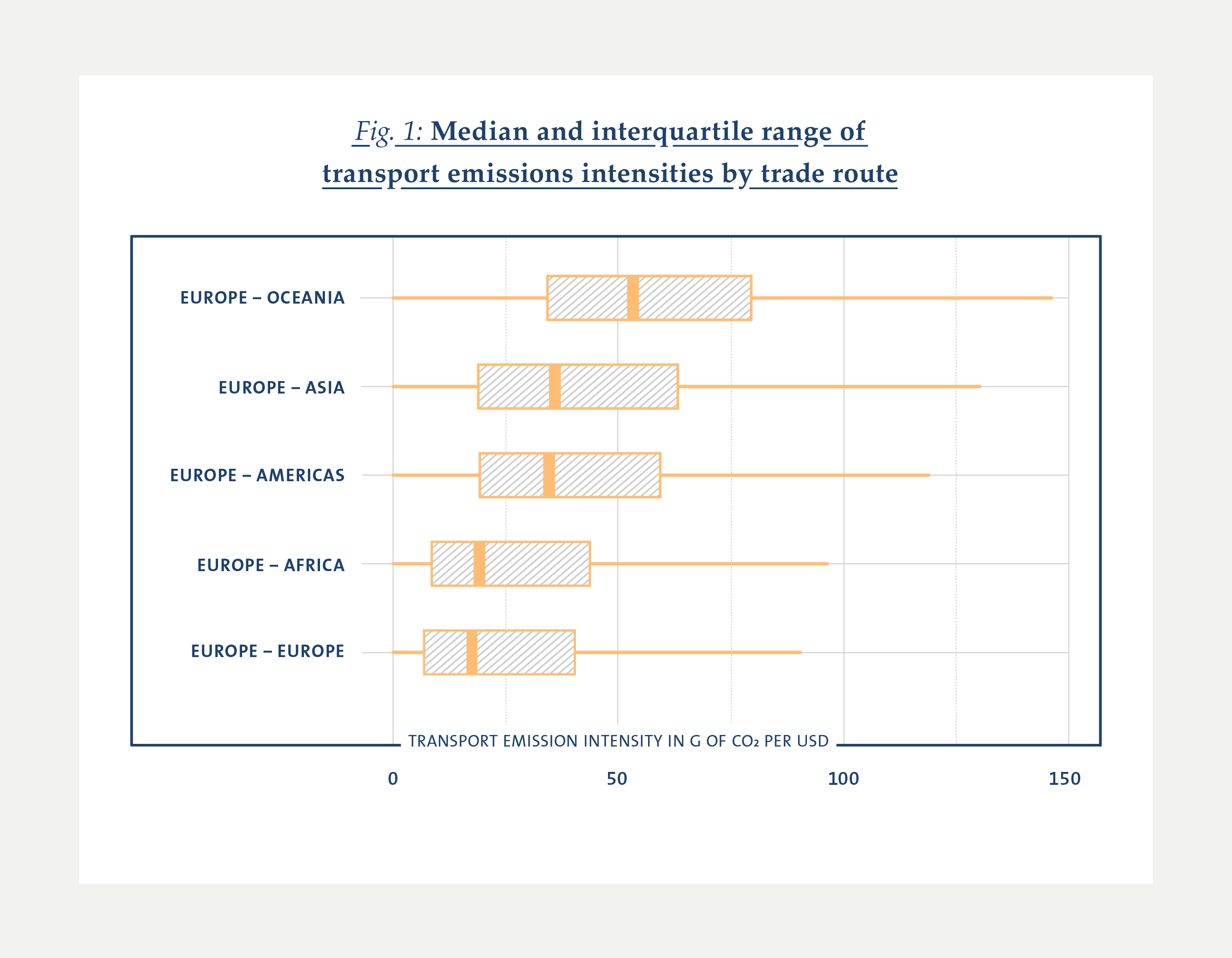
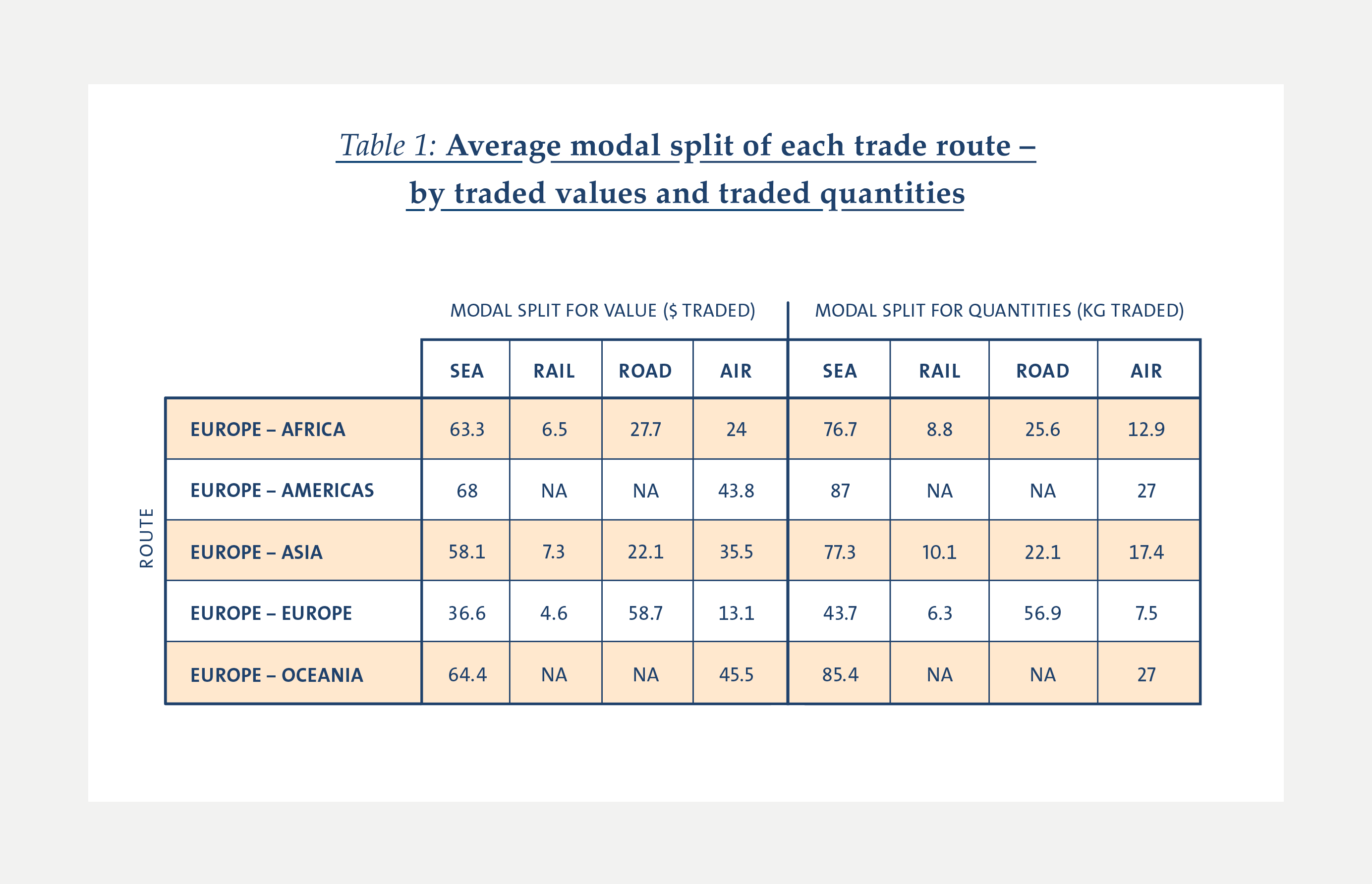
This may arise because of differences in the modal split or the composition of these flows. Transport emissions are highly dependent on the mode of transport used to trade goods for two reasons: (i) differences in emissions per ton-km while everything else held constant, and (ii) differences in the type of goods being transported with each mode. In our example from above, we find that 64% of the traded values between Europe and Oceania is transported by sea, whereas 59% of intra-EU traded value is transported by road (Table 1). A container ship emits on average 10 g of CO2eq per ton-km transported, whereas a heavy-duty truck will emit 76 g of CO2eq per ton-km, tipping the scale in favor of browner modes of transport for intra-EU trade. Once converted in grams of CO2eq per dollar traded, these values become 15 and 37 g, respectively, of CO2eq per dollar, reflecting the higher average value per kg of goods transported by trucks, thereby reducing transport emission intensities in favor of intra-EU trade.
Transport emissions account on average for 16% of total trade emissions.
The contribution of transport emissions to total trade emissions needs to be seen relative to production emissions. For example, the average transaction between Europe and Oceania emits 236 g of CO2 per dollar produced, whereas the average transaction within Europe emits 250 g. Thus, transport emissions will weigh more in trade emissions of the Europe-Oceania route (59% on average) also because what is produced and how is in fact cleaner than in intra-EU trade.
European trade as it is
We now use this database to take stock of European trade as it is. In particular, we compare the total emissions associated with each trade flow with the hypothetical alternative of “buying local”. For each individual trade flow of good g produced in origin o and consumed in destination d, we compare the emissions from production of g in o and transport between o and d in the data in 2015, with emissions from production of g in d with no transport involved.
This exercise is extreme to the extent that not all importers have the capacity of producing the goods that they are sourcing abroad, but it allows us nonetheless to pinpoint where trade makes a positive contribution to reduce emissions. We call a trade flow “green” if the emissions from trade in the data are lower than the counterfactual emissions under local production.8
Our main result is that 28% of European trade flows are already “green” in the sense of bringing about a net reduction in total emissions. This number aggregates the share of green trade flows in EU exports, EU imports, and intra-EU trade. In particular, 34% of all EU exports are green, 22% of all EU imports are green, and 27 % of all intra-EU trade flows are green, according to our definition.
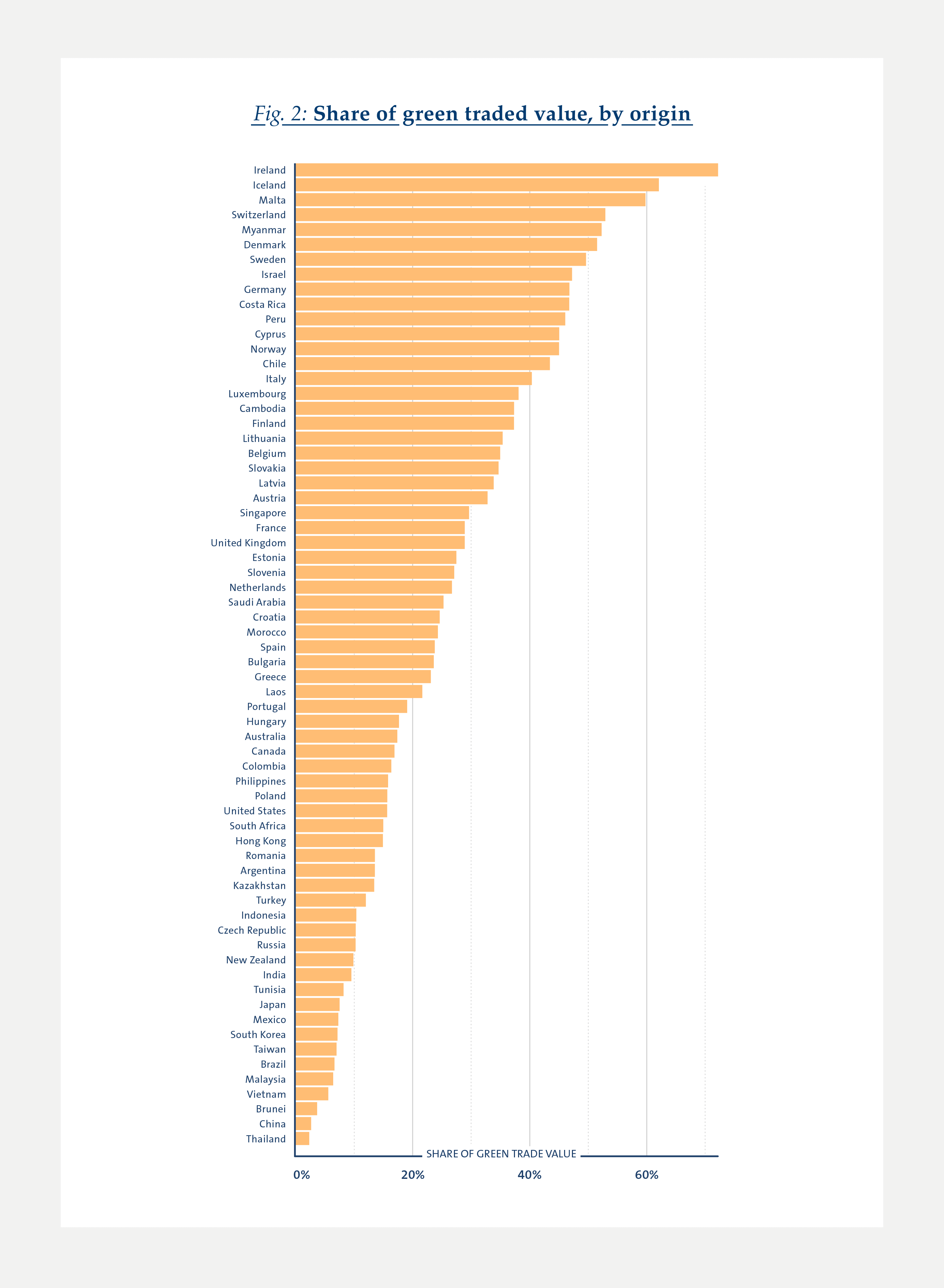
However, green trade flows are very dispersed across origins, destinations, and sectors. Figure 2 reports for each origin country the share of green trade in the total value of their exports. There is a small range of very green exporters (72% of all Irish exports in value are green, 62% of Iceland’s), and a very large range of countries with monotonically declining shares (53% of Swiss exports are green, 47% of Germany’s exports, 16% for the US, 10% for Russia). Southeast Asian exports tend to be very brown with only 2.6% of Chinese exports to the EU labeled green according to our metric.
Green trade flows are very dispersed across origins, destinations, and sectors.
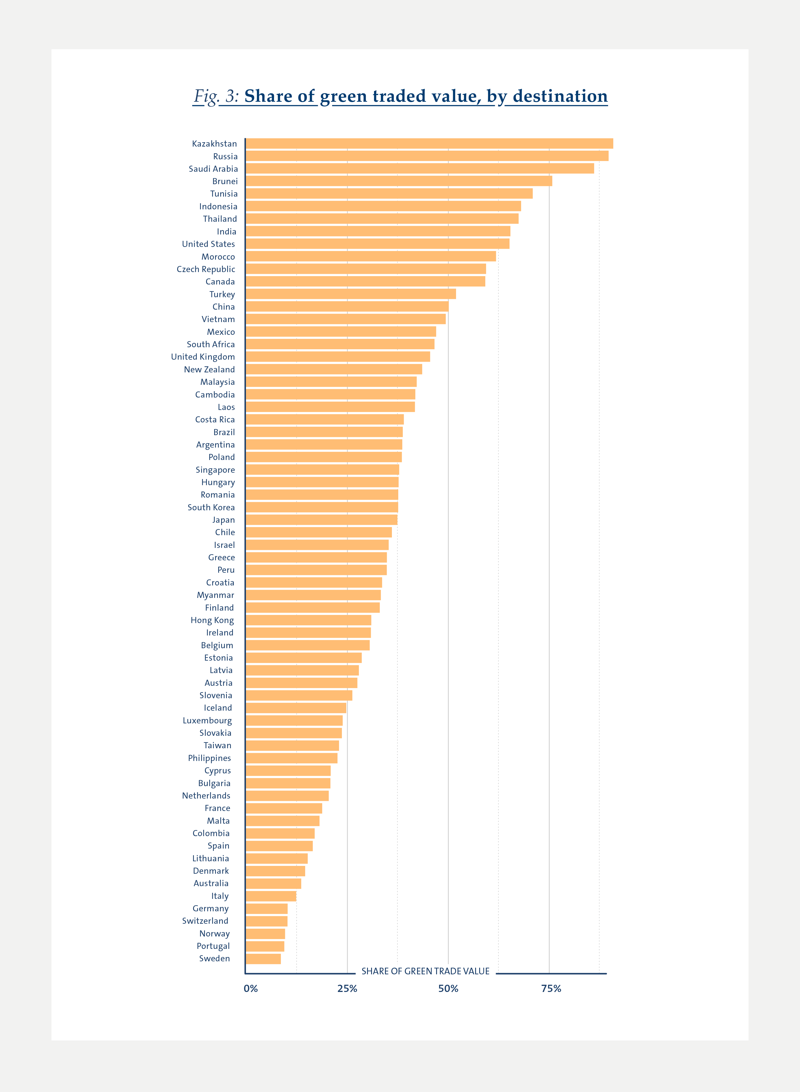
The pattern is somewhat similar when considering importers (Figure 3): 90% of Russian imports are greener if sourced from the EU. Interestingly, 65% of US imports are greener when coming from the EU, whereas this fraction falls to 50% for Chinese imports. At the end of the spectrum for Northern European countries, less than 15% of their imports should be produced abroad rather than locally (10% for Switzerland, 8.6% for Sweden).
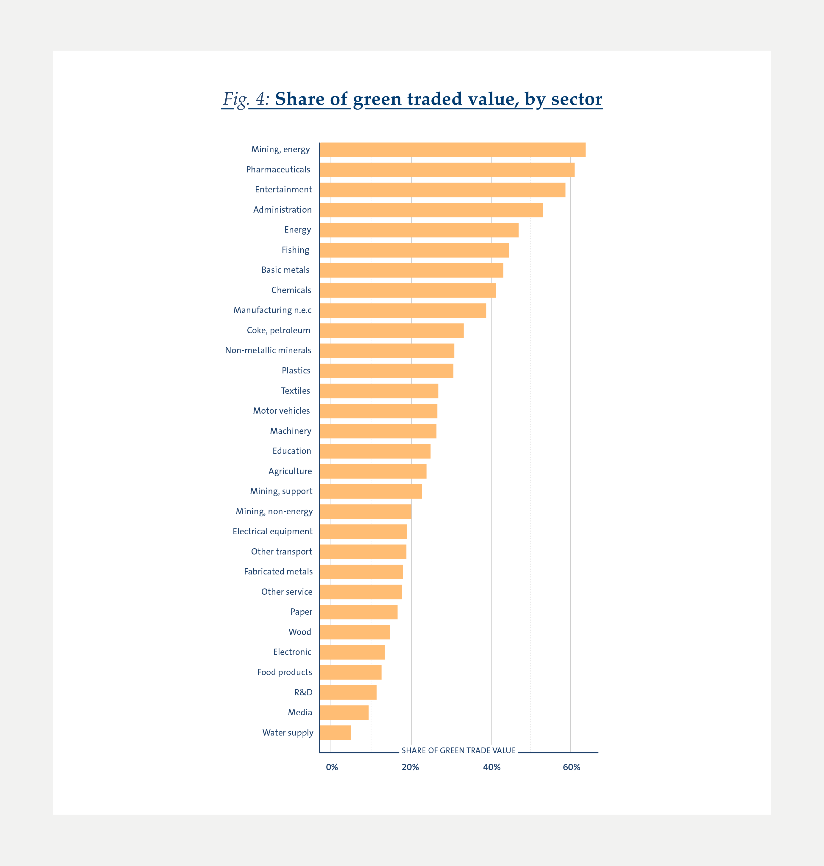
Perhaps surprisingly, the share of green trade value across sectors shows no correlation with production emission intensities. Figure 4 reveals that more than 63% of traded value in the sector of “Mining of energy product” is better traded than sourced locally, with the shares being 61% in “Pharmaceuticals”, 59% for “Entertainment services”, and 53% for “Administrative support activities”. At the bottom of the ranking, only 13% of the value traded in “Food products” is green according to our metric, suggesting that buying local may have an impact in that sector.
European trade as it could be
We now turn to exploring European trade as it could be. In particular, we calculate the emissions reduction associated with a simple green sourcing rule based on a new sector-level metric that we call “foreign green sourcing potential.” A high potential simply means that transport emissions tend to be relatively low and production emissions tend to be relatively dispersed in a sector so that there is a high chance of foreign sourcing being the green choice.
Figure 5 shows what we mean by the foreign green sourcing potential of a sector. Each dot is a sector. The horizontal axis measures the dispersion of the production emission intensities across countries. Other things equal, a higher dispersion comes along with a higher green sourcing potential, since there is then a high chance that foreign countries have access to substantially greener production technologies. The vertical axis measures the share of transport emissions in total emissions. Other things equal, a higher share of transport emissions comes along with a lower green sourcing potential, simply because trading itself is then relatively dirty.
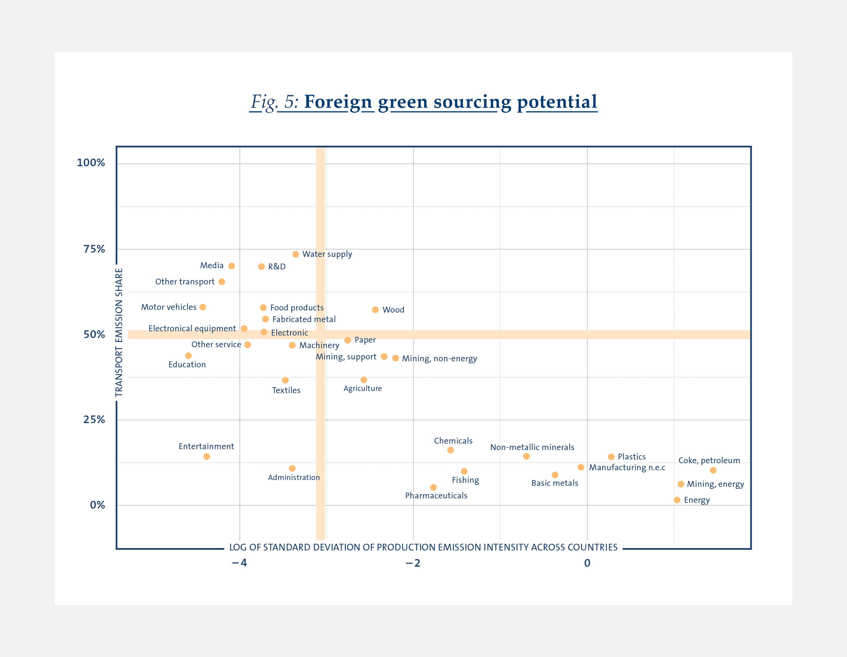
Sectors in the northwest quadrant are sectors with a low foreign green sourcing potential, suggesting that countries should typically source locally in these sectors. This is the case for a majority of tradable services (e.g. “Professional, scientific and technical activities” labeled as “R&D” in Figure 4, which have the second highest transport emission contribution of 70%) that have virtually no production emissions but high transport emissions from individual travel (in the case of R&D, 53 g of CO2 per dollar traded, which ranks in the top 10 sectors with highest transport emission intensities).
Sectors in the southeast quadrant are sectors with a high foreign green sourcing potential, suggesting that countries should typically source internationally in these sectors. It is very interesting to note that amongst these sectors we find raw materials (coke and petroleum, mining, non-metallic minerals) that tend in our data to rank first both in terms of average production emission intensity and production emission intensity dispersion. This illustrates the point made in our previous Kühne Impact Series that the brownest sectors tend to be sourced from the brownest origins, and is at the heart of our argument in favor of green sourcing.
We are now ready to ask by how much emissions could be reduced by going from a world with European trade as it is to a world with European trade as it could be. Our main result is that trade-related emissions could be reduced by 35% if we source goods according to their foreign green sourcing potential.
Concretely, we calculate what would happen to total emissions if countries (i) sourced locally in all sectors from the northwest quadrant of Figure 5, (ii) sourced internationally in all sectors from the southeast quadrant of Figure 5, and (iii) left trade unchanged in all other sectors. In case (ii), we assume that each good transacted in a sector g is now always imported from the globally greenest possible origin o*, that is from a country with one of the lowest production emission intensity for sector g, but with large enough production capacities. In all cases, we also adjust the trade routes to account for changes in transport emissions associated with a change of origin.9
Little effort is required to achieve massive emission savings.
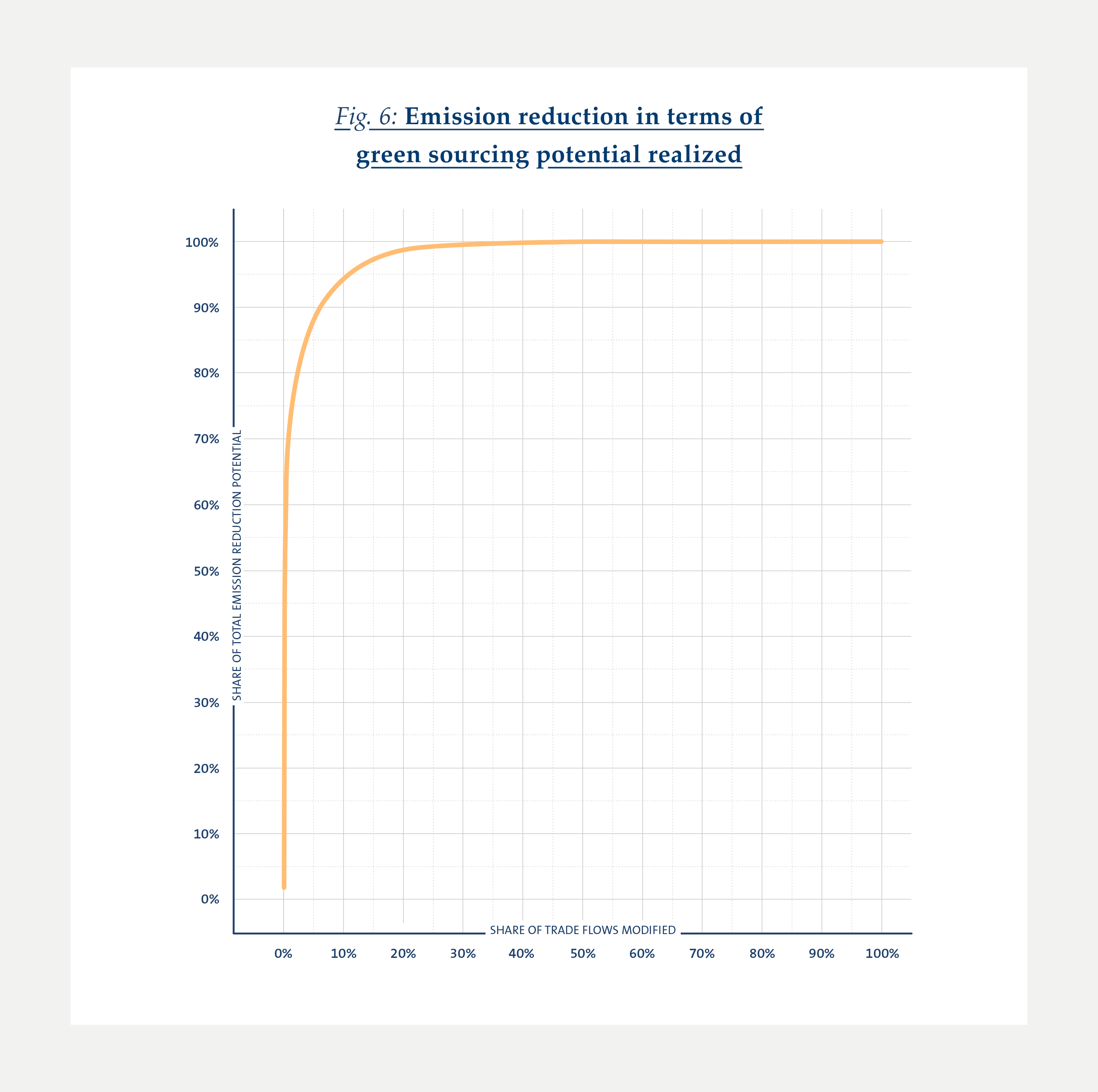
We find that this simple green sourcing rule would reduce trade-related emissions by 35% relative to their level in 2015. Interestingly, much of these gains could be achieved through green sourcing just a small share of critical trade flows. This is illustrated in Figure 6. To construct this figure, we rank trade flows by their “green potential”, that is, by the emissions saved when an individual transaction is being sourced according to our green sourcing rule. We then calculate how much of the 35% emission reduction is obtained when sequentially realizing the green potential of these ranked flows. Figure 6 says, for example, that 95% of the possible emissions reduction through green sourcing can already be achieved by green sourcing only the 10% trade flows where it matters most.
This result reflects the skewness of the distribution in trade emission intensities: a few flows in our data are extremely brown compared to the rest, for example imports of machinery and equipment from China that could instead be sourced from Denmark. This means that little effort is required to achieve massive emission savings.
We can compare this 35% reduction in emission with the gain achieved if one were to “buy local” only. If we impose that any transaction of good g between origin o and destination d is produced locally – by country d rather than country o – we find that trade-related emissions would fall by 14% relative to 2015, less than half of what our green sourcing rule could achieve.10 This confirms the tremendous potential of “buying green” rather than “local” to reduce emissions.
Conclusion
In this Kühne Impact Series, we substantiate our claim that international trade should play a central role in the fight against climate change by providing our most systematic analysis of green sourcing to date. Our main point is that trade can contribute substantially to a reduction in greenhouse gas emissions if sourcing decisions are made by keeping transport and production emissions in mind. Our quantitative assessment is that a simple green sourcing rule imposed on European trade could reduce trade-related emissions by 35% – more than twice of what could be achieved by only “buying local”. Hence, there is a substantial green sourcing potential remaining in European trade.
While we have done our best to keep our quantitative analyses realistic, there is clearly much scope for future work. An important shortcoming of our approach is that we simply impose a given green sourcing rule, instead of studying how the world economy would react to a more realistic policy intervention such as a carbon tax. This is exactly what we tackle in our ongoing Global Sustainability Index project, and we are looking forward to releasing our first results soon.
- “Trade and the greenhouse gas emissions from international freight transport”. 2013. Cristea, A., Hummels, D., Puzello, L. and Avetisyan, M. Journal of Environmental Economics and Management 65, pp. 153–173.
- https://www.oecd.org/sti/ind/carbondioxideemissionsembodiedininternationaltrade.htm
- The Combined Nomenclature (CN) is the primary nomenclature used by the EU member states to collect detailed data on their trading of goods since 1988. It is based on the Harmonized System: The CN corresponds to the HS6 code plus a further breakdown at the eight-digit level defined to meet EU needs. We use the HS6 part. The Harmonized System (HS) classification is an international nomenclature developed by the World Custom Organization for the classification of goods.
- Annex III: Technology-specific Cost and Performance Parameters. 2014. Working Group III Contribution to the Fifth Assessment Report of the Intergovernmental Panel on Climate Change, pp. 1329–1357.
- The original data also includes international trade flows from and to the US that we do not use in this Series. It should be emphasized that the data is still in construction and subject to caveats that we are currently addressing. One of the key limitations to the current data lies in the accuracy of the weights traded. Trade data are not necessarily reported in standard units (tons or kg), and some records were incomplete. When possible, weights were approximated using weight-tovalue ratios at the year-origin-product level (across transport modes). Such ratios are strongly dependent on whether values are measured Free on Board (FOB) or including “Cost, insurance and freight” (CIF). European imports, for example, are all reported in CIF. This means that the monetary value of these flows includes the cost of the transport, and as such is overestimated. As a result, imputed weights will be underestimated. The emissions reported in this Series should therefore be viewed as a conservative estimate of transport-related emissions.
- See our Kühne Impact Series “Buy Green not Local: How International Trade Can Help Save Our Planet” (03/2021) for a detailed discussion of heterogeneity in emission intensities
across producing countries and sectors. - See our Kühne Impact Series “The European Green Deal: Transforming International Trade and Transportation” (12/2021) for a discussion of the European propositions on carbon taxation.
- Note that in the cases where a country simply cannot produce a good locally (e.g. for raw materials) it will be the case that in fact we don’t have a production emission
intensity for that country (since there is no output). These instances are rare given the coarseness of the data (0.7% of the country-sector pairs in 2015). When that is the case, both the original trade flow and the counterfactual emissions are dropped from the comparison so as not to bias the main message. - To keep this exercise as realistic as possible, we adopt a certain number of rules to allow a country to be considered as potential sourcing origin (mainly that they already have a large output). We also need to adjust transport modal split to reflect the new routes. See the technical appendix for an exact description of our sourcing rules, and the methodology adopted to construct counterfactual trade flows and emissions.
- To avoid cases where a country would be forced to produce something it never has before, we impose again some restrictions on the sourcing patterns. If a country has no
capacity to produce a sector, be it because observed gross output is too low or because of natural resources constraints, we impose that sector g be sourced from a close neighbor in terms of geographic distance. See details in the technical appendix.


More Issues
Variable Carbon Pricing and the Environmental Gains from Trade
Optimal Carbon Tax for Maritime Shipping?
The Global Diffusion of Clean Technology

The Sustainable Globalization Index

The Distributional Effects of Carbon Pricing:

The Green Comparative Advantage:
Global Trade

The EU Emissions Trading System

The European Green Deal

Post-COVID19 resilience

Africa’s Trade Potential

Buy Green not Local

A New Hope for the WTO?

Crumbling Economy, Booming Trade
Pandemic and Trade
The Dynamics of Global Trade in Times of Corona

EU Trade Agreements
Past, present, and future developments