Impact Series: 05-23
Optimal Carbon Tax for Maritime Shipping?
Environmental Policy meets Network Economics

Outline
The world trading system is a very complicated network comprised of shipping routes that link many connecting ports or nodes. In such a networked setting, the economics of regulation is challenging because the efficiency of a networked system depends on both the set of active nodes (ports) and the volume of activity flowing through its links (trade). In this Kühne Impact Series, I discuss how a standard environmental policy such as taxing carbon emissions may have the unintended consequence of lowering overall network efficiency. As a result environmental policies need to be designed carefully whenever network interaction effects are large. When they are large and positive, as seems to be the case, then the optimal carbon tax is below the marginal social cost of carbon.
Introduction
International shipping connects over 200 countries, via thousands of ports, to convey perhaps 80% of world trade (by volume). It is critical for the functioning of the global economy and offers a path to development for many distant and commodity-rich developing countries. Although somewhat polluting, maritime shipping generates the lowest carbon emissions per ton/km of all available transport modes.
It is also true that the structure of world trade represents a network connecting nodes (ports/countries) via links (shipping routes/trade), and therefore, shocks to one part of the network can, and sometimes do, dramatically reverberate elsewhere in the world economy. There are many recent examples of these long-armed network effects: the disruption created by the container ship Ever Given being stuck in the Suez Canal; the large supply chain disruptions created by the Covid pandemic; and closer to home for most people – the local airline delays created by violent storms in faraway regions or countries. Economists have been aware of network effects for decades, but the formal analysis of network economics in transportation began only in the 1990s when U.S. deregulation of passenger air travel led to concerns over flight availability and antitrust issues. Network economics is now a thriving, very large, and very complicated branch of applied microeconomics.1
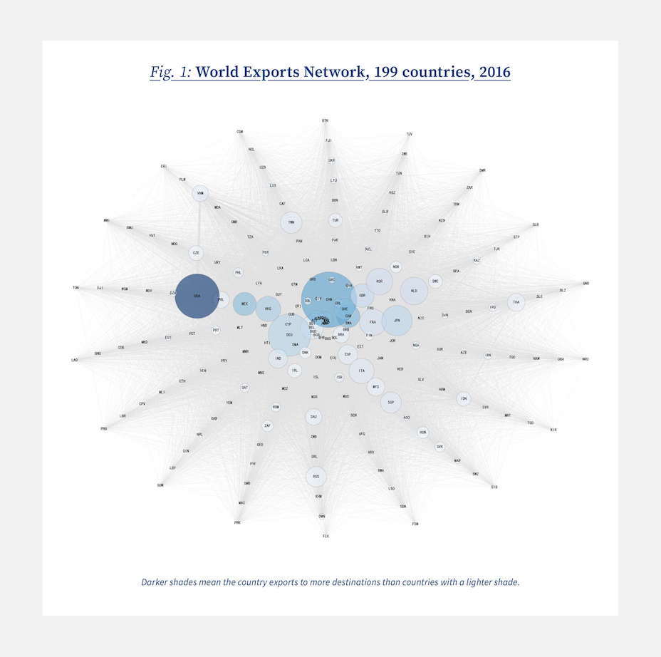
The world trading system is surely one of the most important networks in the world. Its geographic scale is unparalleled, and in volume terms alone, it transported over 25 trillion U.S. dollars of exports in 2022. Naturally, it is difficult to appreciate the complexity of the countless connections this implies, but we can at least visualize them. In Figure 1 I present a network graph where light grey lines connect every pair of countries that trades with each other. These lines represent the network’s links. Countries, which are the network’s nodes, mostly appear as dots, but relatively large exporters are shown as bubbles (containing their 3-letter country code). The size of these bubbles is proportional to the dollar value of their exports. As a result, China – the world’s largest exporter – has the largest bubble, and is followed by the U.S., Germany, Japan, etc. The color of the bubbles is also informative. Darker shades of blue mean the country exports to more destinations than countries with a lighter shade. So for example, the U.S. exports to more countries worldwide than any other. The star pattern means nothing at all; it was selected for esthetic and not economic reasons.
The world trading system is a connected network: Any disruption or expansion of trade in one part of this network will ripple through the entire system.
Finally, although it is virtually impossible to see – no country is isolated. Even the pariahs of the world economy trade with someone, who trades with someone else, who trades with ... This tells us that the world trading system is a connected network. As a result, the figure is especially useful in conveying an idea that statistics alone cannot: any disruption or expansion of trade in one part of this network will ripple through the entire system. I call these knock-on effects created by shocks, network interaction effects.
But why do these network interaction effects exist, and what does their existence have to do with environmental policy?
Defining a Network
While it is easy to see how ports and shipping connections across countries represent a network of sorts, to an economist, a network means much more than just connections across economic agents. Our entire economy is to some extent a network in this sense. More formally, we typically identify a networked setting as one with three key features.
First, there is a group of agents (individuals, shippers, etc.) which we think of as being located at points or nodes, and this group interacts in some way along links created amongst them. These could be physical linkages like shipping routes between ports; they could be ephemeral links created via the web or online platforms; or they could be financial flows across a financial system; but all networks must have nodes and links. We tend to think of nodes as decision points, and links as representing the flow of outcomes from these decisions.
Second, the benefits of being part of a network are increasing in the number of participants. So if B(N) is the benefit (monetary, psychological, or social) a member receives by being in a network when it has N members, then we would say B(N + 1) ≥ B(N) ≥ B(N − 1). Bigger is better. Being part of any social media platform has this feature: it is easier to learn about new music or be entertained by funnier cat videos if your social network has 1 billion rather than 1 million people in it. In the trade context, we think of ports and their shipping routes as the global trade network; and the benefits of this network to participants should be rising in the number of participants. For simplicity, I call this the membership benefit of networks.
The third, and related feature, is that the benefits of being a member in a network, of any size, are typically rising in users’ activity. Again, in the social media context, it is better if users are active in posting and responding to materials than if they are relatively silent. And in the trade context, adding a potentially busy port to the worldwide trading network is more important than adding a quiet one. We could call this the activity effect, and expand our notation to include these new benefits of network activity X so that for any network of given size N, the benefits of being a member of this network are higher when agents are more active X. Formally, we would have B(X′′,N) ≥ B(X′,N) ≥ B(X,N) whenever X′′ ≥ X′ ≥ X. For simplicity, I call this the activity benefit of networks.
It is important to recognize why the economic structure of networks, can and often does, present unique challenges for regulators – be they antitrust regulators wanting to ensure competition amongst airlines or environmental regulators wanting to constrain carbon emissions. The reason is simply that when an industry exhibits these properties, individual agents working within the network make decisions that are, to some extent, less than socially optimal. The reasons for this are simple. When I decide to join a network, I do so because my personal benefits of joining exceed my personal costs. I do not take into account the external benefits I am creating for others via the membership effect. This benefit is completely left out of my calculation, and therefore, membership is, in general, too low.
Similarly, when I post an advertisement for an item to sell on a social-media-sponsored market (for example Facebook Marketplace), I do so because it is expedient for me to do so. When making my decision I don’t take into account that other potential sellers, seeing how popular this marketplace has become, also choose to place their ads in the same place. Greater activity means it’s now easier for buyers and sellers to meet – transaction costs are lower and the marketplace is more productive – but I surely didn’t take this into account when I decided to post my ad. As a consequence, despite how popular social media marketplaces can be, there may in fact be too little activity on these networks.
To understand why network interaction effects should matter to policymakers, we need to take a step back to understand the basic economics guiding environmental policies.
Therefore, almost by their very design, networks create both membership and activity benefits for parties external to individual decision-makers. In economics, we would say they create positive externalities. And in an economic system where participants are linked and their decisions create positive externalities, disruptions or shocks to one part of the system will create knock-on effects elsewhere; that is, they create what I referred to earlier as network interaction effects.
To understand why network interaction effects should matter to policymakers, we need to take a step back to understand the basic economics guiding environmental policies. We start with a situation where there are no network interaction effects and then ask how their addition would matter for the design of environmental policy.
Economics 101: A Market Equilibrium
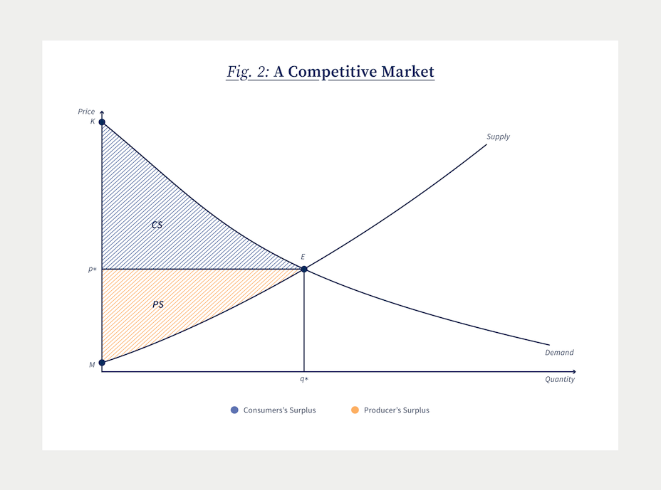
The simplest way to convey how network economies can matter to environmental policy is to discuss a simple textbook example (readers with an aversion to graphical analysis can skip directly to the bolded summaries in this and the next section). To help with this discussion I construct the demand and supply apparatus economists use to discuss market outcomes in Figure 2. As shown, it contains an upwardly sloping supply curve labeled S, and a downwardly sloping demand curve labeled D. Each of these curves represents a list or menu of choices: quote me a price and I will tell you the quantity I want to demand (consumers) or am willing to supply (firms). Their intersection at point E is where the quantity demanded by consumers exactly matches the quantity supplied by firms, at the quoted market price, p*. Since the quantity demanded at that price equals the quantity supplied, we call this the equilibrium price. Also shown is the equilibrium quantity q*, and I have labeled two points on the vertical axis M and K. Ignore for the moment the shaded areas.
The price p* brings demand and supply into balance. At any higher price the quantity demanded by consumers is smaller; but at this higher price the quantity supplied by producers is bigger. Too much supply and too little demand would lead to prices falling which would in turn reestablish the price p where they are once again in balance. This is of course why we call it the equilibrium price.
Apart from identifying the equilibrium price and quantity in a given market, economists also use this diagram to talk about the benefits provided by free competitive markets like this one. We associate the vertical height of the demand curve, at any given quantity, with the maximum willingness of consumers to pay for that quantity of the good. It is easy to see that willingness to pay is greatest when the quantity of the good being offered is small (near the vertical axis), and if we push this quantity even smaller to point K, we find consumers’ highest willingness to pay.
An immediate, but not necessarily obvious, implication of this analysis is that in the Market Equilibrium, consumers are getting a great deal. They are paying p for every unit of the good consumed, despite the fact that their maximum willingness to pay is in general far higher than p*. We define this gap between what consumers would be willing to pay, the vertical height of the demand curve, and what they have to pay in the market, which is p*, Consumer’s Surplus. We measure its magnitude in any market by an area like the triangle shown with vertices K, E, and p*. In total, it represents the benefits consumers reap from the existence of this market.
Now turn to the firms supplying this good. The supply curve represents, at each quantity, the minimum price firms would need to supply that quantity of goods to the market. The supply curve is upward-sloping because bringing more and more of a good onto a market will be increasingly costly to firms. More workers will be needed, overtime hours may be required for production, and firms may need to hold more inventory. For all of these reasons, these marginal production and delivery costs rise with the quantity supplied, and therefore, firms need higher prices to compensate.
Now consider the benefits firms get from participating in this market. The supply curve measures the minimum price needed to convince firms to supply a given quantity of the good. For very small quantities supplied, firms are ready to accept relatively low prices. The lowest price consistent with some supply is at the hypothetical minimum point M. As quantities grow, the supply curve rises reflecting an increasing marginal cost of supplying additional units. But at the equilibrium price p*, firms are supplying the vast majority of their output at a price well over the minimum they might accept. This gap between the equilibrium price p and the minimum acceptable price is called Producer Surplus. It is given by the yellow shaded triangular area defined by the vertices M, E, and p*.
I would like to make two final observations on the Market Equilibrium model before we discuss environmental policy. First, it is useful to note that no other price, other than the equilibrium price p*, would maximize the sum of Consumers’ and Producers’ Surplus. At any higher price the marginal cost of producing goods (the height of the supply curve at the greater quantity) is greater than the marginal benefit (the height of the demand curve at the greater quantity). This means that even a well-meaning government could not improve on this market outcome. The market got it right. It already provides the greatest benefits it can to society because, surprisingly, the decisions made by self-interested consumers and producers have unwittingly generated this outcome. As a consequence, the supply curve which reflects the marginal cost of production to private firms also represents the marginal social cost of production (MSC); and the demand curve which reflects the marginal willingness to pay for private consumption – also represents the marginal social benefit (MSB) of consumption. This last point – that the market got it right – was, of course, made much more eloquently by Adam Smith over two centuries ago, and has been the philosophical foundation for a belief in the welfare-maximizing powers of free and competitive markets ever since.
Our final observation comes in the form of a question – where does all that Producer Surplus go? The astute reader will notice that total revenues to firms are given by the rectangle (not drawn) defined by p* times q*, and the area of this rectangle is larger than the sum of the marginal costs firms incur when producing q* (this is measured by the area under the supply curve up to q*) which is their total (variable) costs. So is this difference firm profits? The answer is that in a competitive market, Producer Surplus represents the return that firm owners receive on their past investments in plant and equipment. If Producer Surplus was larger, their return on capital would be greater; if it was smaller, their return on capital would be smaller. Implicitly, the figure assumes firm owners are happy with the current state of affairs because the competitive rate of return they are earning is as good as they are going to get elsewhere. If not, they would have left the industry already.
A competitive market is in equilibrium when the quantity demanded equals the quantity supplied.
Summarizing
A competitive market is in equilibrium when the quantity demanded equals the quantity supplied. Competitive markets maximize the sum of Consumer and Producer Surplus by ensuring that the social costs and social benefits of the last unit produced are equated. This equilibrium could continue indefinitely because firm owners are earning a competitive rate of return on their investments in plant and equipment.
Environmental Policy 101: A Regulated Equilibrium
To discuss the impact of environmental policy we need a reason for policy, so let’s assume each unit of the good a firm produces also emits one unit of pollution. To be current, let our pollutant be carbon. And note that, at least in the short run, firms have very few ways to abate carbon. It typically takes time and new investment to move away from carbon-intensive energy by altering fuel choices, technologies in place, etc. So, I assume that for our purposes, the only way to abate carbon is to produce less output. Finally, what is the cost of these emissions to society? Since carbon is emitted worldwide and by many industries, it is reasonable to think the marginal cost to society for the emissions produced in our one industry is effectively a constant. I will refer to this constant per unit cost of carbon as C, and in the parlance of environmental economics, C is the marginal social cost of carbon. The existence of this cost means there is now a gap between the private and social costs of production. This is the raison d’ être of environmental policy.
With these preliminaries out of the way, consider the figure below, where I have constructed a Regulated Equilibrium. In many ways, the Regulated Equilibrium replicates the Market Equilibrium just discussed. Equilibrium is reached when the quantity supplied equals that demanded, and we can again measure Consumer and Producer Surplus similarly. But the figure below is, of course, complicated by not one but two supply curves, two shaded areas, and three different prices that are labeled. Ignore all of these additions and start by noticing that our Market Equilibrium supply and demand curves, S and D, are just repeated in the figure. Their intersection would again generate a Market Equilibrium with the price of p and quantity q*. So far, so good.
But now, shift your focus to the curve labeled MSC and recall that the height of firms’ supply curve represents their marginal cost of production. If we add to the firms’ private costs of production the social cost of the carbon also emitted by production, then we obtain what is known as the marginal social cost of production as shown by MSC. By construction, this curve only differs from the original supply curve by adding the social cost of carbon C.
Suppose there is no environmental policy, and firms are free to emit as much carbon as they like. Then we are back to our Market Equilibrium outcome at E. But notice at E the benefit to society from the last unit sold, which is given by the vertical height to the demand curve at E, is now well below the marginal social cost of this last unit, which is the vertical height to O. This means this last unit of production cost society more than it was worth to society. In fact, for all units of production beyond qR there is a gap between marginal social costs and benefits. And because costs exceed benefits over this range, the blue shaded triangular area with vertices O, S, and E has an area equal to society’s losses because too much carbon is emitted in the Market Equilibrium.
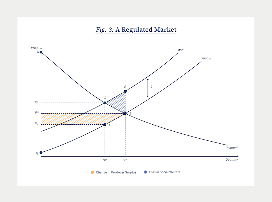
The solution to this is simple in theory. One possibility is to introduce a carbon tax on emissions. If the tax per unit of emissions equals C, then the firm’s full costs would be equal to their production costs plus their costs from paying the emissions tax. This means their willingness to supply output to the economy would then be reflected in their new supply curve, which is the curve labeled MSC for marginal social cost. Equilibrium in the Regulated Market would occur at S.
Consumers would consume qR units paying pD for each unit. Firms would also receive pD but they also need to pay their carbon tax of C on each unit sold. Therefore, the price firms actually get for supplying qR units is only pD − C = pS as shown. Notice that at the new Regulated Equilibrium, we have successfully balanced the marginal social costs of production to the marginal social benefit of the last unit sold. No other policy is required. A simple carbon tax solves the problem and generates an efficient solution.
Despite this efficiency, the level of economic activity in this industry has fallen. The output of firms is smaller with the carbon tax in place. Moreover, the price firms receive (net of the carbon tax) for each unit of production is now lower than previously. Together, these adjustments mean that Producer Surplus of firms falls by the yellow shaded area in the figure with vertices A, E, pS, and q*. All else equal, this means that the owners of plant and equipment in the industry earn a lower rate of return than they did previously. This reduction may lead to their exit from the industry. In fact, one of the most common arguments firms make against a simple carbon tax plan like the one shown is that it will effectively drive them out of business because it lowers their return on investment. Simple economics supports this claim.
The price consumers have to pay for the good has also risen with the carbon tax. As a result, they lose some Consumer Surplus (not shown), but they also benefit from the fact that carbon emissions are now lower (also not shown). But not everyone can lose because society as a whole gains from the imposition of the carbon tax: notice that the government (which is part of society!) collects carbon taxes equal to the rectangle with vertices pD , S, A, and pS. Whether firm owners or consumers win from carbon taxes depends on how governments distribute or recycle this revenue. For example, the government could rebate it to consumers by sending them checks in the mail; they could instead use the tax revenues to pay for other public goods; they could use the revenue to lower taxes elsewhere while keeping their budgets in balance; or they could instead rebate revenues to firms. The possibilities are endless.
Policy makers have to ask whether the imposition of the carbon tax in one market has important knock-on effects in other markets.
While there are a myriad of options, we now know that how governments recycle their carbon tax revenues matters not only for the distribution of costs and benefits of the policy, but also for the wider economy’s overall efficiency. This is a critical point. It follows for an obvious reason but the complete argument is a little subtle. We know that any real-world economy has many taxes in place because governments must raise revenues for the provision of public goods like education, transportation, health, etc. However, some of these taxes create large gaps between the costs and benefits of private transactions. This is inefficient for the economy as a whole. We might think of lowering these especially inefficient taxes and use our carbon tax revenues to make up the difference. This is called revenue recycling, and if those new carbon tax revenues exactly offset the losses we incur by lowering those other inefficient taxes, we call it a revenue neutral carbon tax plan. Revenue recycling is, not surprisingly, a good thing for the economy. But there are limits to how good. Since carbon taxes are primarily energy taxes, they affect almost all sectors of an economy, and policymakers need to worry about how carbon taxes interact with those existing inefficient taxes (or distortions). They have to ask whether the imposition of the carbon tax in one market has important knock-on effects in other markets. By that, we mean, does it make the existing inefficiencies created by our tax system even worse?
If so, our calculation of the costs and benefits of the simple carbon tax shown here needs to change. In the economics literature these knock -on effects are called the tax interaction effects and they are the added costs or benefits that arise elsewhere in the economy when we impose a broad–based carbon tax. Tax interaction effects have been studied extensively, but in a nutshell, they are almost always costly to the economy and their costs are larger than any benefits we might get from revenue recycling. As a result, the existence of tax interaction effects argues for a lower tax on carbon emissions than the C we imposed here. It has to be lower because of those net negative knock-on effects.2
Tax interaction effects are almost always costly to the economy and their costs are larger than any benefits we might get from revenue recycling.
Summarizing
In the Regulated Market Equilibrium, the quantity demanded equals the quantity supplied. When the carbon tax is set equal to the marginal social cost of carbon, and there are no tax interaction effects, this equilibrium is efficient. The marginal social cost of the last unit of production equals its marginal social benefit. The carbon tax increases overall welfare to our society (CS, PS, and tax revenues), but can create both winners and losers. In the absence of tax rebates or similar adjustments, the producers will see a reduction in Producer Surplus and a lowering of the rate of return earned on their investments in plant and equipment. Firms may exit the industry as a result. When tax interaction effects are present, they imply the efficient carbon tax is below the marginal social cost of carbon we identified as C.
Implications for Maritime Shipping
Let’s now assume that network interaction effects are present in maritime shipping. These effects could come from either, or both, of the underlying membership and activity benefits common to network settings. Let’s also interpret the supply and demand curves previously shown in terms of shipping services for bulk commodities.3
Specifically, let the demand curve be the demand for shipping services from producers at port A wanting to deliver their goods to port B. Let the supply curve represent the increasing number of bulk ships willing to make the voyage from A to B as the price they receive for the trip rises. Before the carbon tax is implemented, the number of voyages made is q*. After the carbon tax is implemented the volume of shipping falls to qR; that is, shipping activity to port B falls.
If ports A and B are part of a wider shipping network that exhibits a positive activity externality, this reduction will lower productivity elsewhere in the network. For example, with the activity at port B now reduced because of the carbon tax, commodity shippers at port B may have a very hard time finding a bulk ship to carry their own cargo onward from port B to some other port C. The beneficial trades that would have occurred between shippers in B and ship owners with ships present at port B, will now not occur because fewer trips and ships now land at B. This reduction in activity has a social cost and constitutes a network interaction effect of the carbon tax.
In addition, the ship owners that do carry goods from A to B, reap a smaller Producer Surplus from their voyage than previously. Note their fuel plus tax costs are now higher with the carbon tax. This implies their return on capital is now lower, and when it is time to scrap their ship and reinvest, they may not do so. The fleet, whatever size it may have been, is smaller as a consequence. This can mean that smaller, marginal ports that were profitable before the tax was implemented, are no longer profitable now. Ports may close and membership in the network falls. These changes can also create productivity losses, and therefore are also part of our network interaction effects.
In summary, the full impact of a carbon tax on the maritime shipping industry consists of the change in Consumer Surplus, producer surplus and tax revenues collected by governments, but we must also consider – how the carbon-tax-created network interaction effects – lower social welfare elsewhere. A reduction in network size or activity creates negative network interaction effects, and this suggests our simple carbon tax at level C is too high.
Do Network Effects exist in Maritime Shipping?
The argument thus far begs an important question: do network externalities exist in global shipping, and if so, do they create network interaction effects? The answers we have come from three different approaches. One approach relies on indirect evidence of the strength of network effects. This evidence is obtained by taking a given network and investigating its statistical features. For example, when network externalities exist they tend to produce outcomes where the majority of activity is concentrated in only a few nodes (ports), with many other nodes (ports) far less active. This bunching or concentration of activity is a phenomena often associated with the name of Italian polymath Vilfredo Pareto (1848–1923) who just happened to be a Professor of Political Economy at the University of Lausanne. It is Pareto who is responsible for the Pareto principle (20% of the Y deliver 80% of the Z). This observation was subsequently formalized in the Pareto distribution, which bears his name and exhibits this same feature. Discovering that a network’s activity is distributed across its nodes in a Pareto fashion does not prove there are strong network externalities, but the finding is consistent with and suggestive of them.
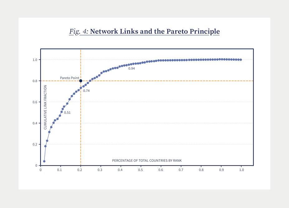
To illustrate this Pareto feature we can use the same world trade data shown in Figure 1 to present a figure that relates the number of country-to-country trading links a country has (perhaps its 130) to its place in the world ranking of active nodes (this number of links would put it in the top 5 countries). To turn this information into a distribution – that we can relate to Pareto – we need to use percentages rather than raw numbers, and its best to show the outcome in a graph. In Figure 4, we plot the percentage of unique country-to-country links on the vertical axis against, the percentage of countries ordered by rank that have those links. The black dot could be called the Pareto point. It represents the point where countries in the top 20% by rank trade along 80% of the world’s links. It’s important to recognize that our data may or may not fall anywhere near the Pareto point, but by construction, the dotted line shown must go through both the origin and then rise to point (1.1) at the top right corner. Beyond this, the shape is entirely determined by the data.
One thing is obvious. The set of trading links is highly concentrated. The U.S., China, and the EU would for example capture the lion’s share of all routes/links in the data. In fact, reading vertically up from the point at .1 on the horizontal axis, we find that countries in the top 10% (by rank) trade along on 51% of all the routes/links (the .51 in the label bubble). Reading up using the yellow dotted line, we see that the countries in top 20% trade along 74% of all possible routes/links (and note how close this result is to the Pareto Principle requirement of 80%). Finally if we read up from .4, we find that countries in the top 40% account for 94% of all routes/links. This is overwhelming evidence that worldwide shipping links are highly concentrated across countries. This first piece of evidence is highly suggestive of network effects.
A second, more direct method to investigate network effects is to use shipping data to evaluate whether the historic pattern of worldwide maritime shipping exhibits network features. For example, Kosowska-Stamirowska (2020) uses machine learning algorithms to predict both the flow of trade between port pairs and the likelihood of a new trading link being created between existing ports. She finds a very basic feature of network architecture – the number of common neighbors any two ports have – is the strongest predictor of trade flows and the likelihood of a direct trade route existing. This implies that shocks to the system – natural occurring shocks or policy created shocks – that affect the number of nearest neighbors for any port, will ripple through the entire structure; that is, they will create network interaction effects.
Finally, while these two pieces of evidence are suggestive of strong network effects, they do not estimate them. To take this last step we need to find an explicit connection between features of world trade and the strength of network externalities. Recent work by Heiland et al. (2019) does just that by using an explicit model of trade within a spatial network. They find very significant positive network externalities within the global trading system. This implies, therefore, that negative policy shocks will have knock-on effects elsewhere – network interaction effects are real – and can create significant social costs that are not accounted for in our standard economic analysis.
The next step is to find an explicit connection between features of world trade and the strength of network externalities.
Conclusion
The international trading system relies on a healthy and vibrant maritime shipping industry to deliver goods worldwide. For countries far from the richest markets and with exports that are of the lowest value to weight, disruptions to this industry will be costly. These are primarily developing countries who are relying on trade as an engine of growth and a path to prosperity. It is then especially important we get any environmental policy affecting the maritime sector right, because the costs of not doing so will fall disproportionately on poor nations.
In this note, I have suggested that the structure of world trade can best be thought of in terms of a network where ports serve as nodes and the flow of traded goods carried by vessels represents their links. In network settings like this one there are often external benefits (externalities) created by either increases in activity (the flow of trade) or increases in their membership (the entry of new ports). When these network externalities exist, any shock to the system – whether positive or negative – flows through the network via what I have called network interaction effects. In general, both positive and negative shocks are magnified because of the positive externalities inherent in the network structure.
The immediate and important implication of this is that our standard textbook solution to internalize the social cost of carbon emissions is unlikely to hit the mark. When a carbon tax lowers network activity and makes ports less profitable, it will have knock-on effects with negative social costs. All else equal, the optimal carbon tax will be lower than otherwise. This result mimics well known results in environmental economics where tax interaction effects in economies with existing distortions lowers the optimal carbon tax below the Pigouvian (C in our context) level.4 It is also important to recognize that while I have presented this argument using a carbon tax, less efficient environmental measures – such as technological requirements or performance standards – will work slightly differently but will also create network interaction effects. Land-based transport and air transport may also exhibit these effects.
All of these conclusions follow when significant and positive network externalities characterize the world trading system. While the evidence at this point in time is fragmentary, it is also suggestive. The distribution of network links is well approximated by the Pareto distribution tied to network design; existing network structures predict trade flows and port creation very well, and estimates of the international externalities within the world trading network are positive.
The way forward is clear. Researchers and policymakers alike need to focus on understanding the economics of environmental policy in networked settings. We should ask how common network interaction effects are in the economy overall, and we should be developing empirical methods to estimate their size. Environmental policies need to be designed carefully whenever network interaction effects are large. When they are large and positive, as seems to be the case, then the optimal carbon tax is below the marginal social cost of carbon.
- See the recent book length treatment of Goyal (2023). Important early work on network design in transportation is Hendricks, Piccione and Tan (1995).
- The most well-known example of these tax interaction effects is examined is Bovenberg and Goulder (1996). They show that in the presence of another distortion in the economy (a distortionary labor tax), the optimal carbon tax is significantly lower than the Pigouvian level C shown in our figure. Exceptions to this rule are discussed in Goulder (1995).
- The market for bulk cargo shipments and vessel trip supply does not operate like the smoothly operating demand supply analysis we have constructed. Instead shippers and ship owners search for partners and negotiate over prices. A model of bulk shipping with explicit search and negotiation is Brancaccio, Kalouptsidi and Papageorgiou (2020). None of these real-world complications alters the basic point I will be making.
- The problem I have described here is well known to economists. If there are (unrealized) network economies in world shipping AND shipping emits carbon, there are two problems for government policy to address and not just one. As a result, the efficient solution almost always requires two policies, and addressing only one of the problems while ignoring the other may even make matters worse by creating negative network interaction effects. This is perhaps the most important implication of the seminal work of Lipsey and Lancaster (1956) on the General Theory of Second Best. In our simple context, one solution is to use a carbon tax to internalize the social cost of carbon, but we also need to internalize the social benefits of network expansion by subsidizing port construction (because of membership externalities) and facilitate higher volumes of shipping (because of activity externalities). Even if these subsidies exist, we need to coordinate their level and adjust their strength with the introduction of a carbon tax for the solution to be efficient. In the absence of coordination, the second-best policy is to let one of the instruments (a carbon tax) deviate from what it would have been otherwise. In our context, it would be lower.
- Bovenberg, A Lans, and Lawrence H Goulder. 1996. “Optimal environmental taxation in the presence of other taxes: general-equilibrium analyses.” The American Economic Review, 86(4): 985–1000.
- Brancaccio, Giulia, Myrto Kalouptsidi, and Theodore Papageorgiou. 2020. “Geography, transportation, and endogenous trade costs.” Econometrica, 88(2): 657–691.
- Goulder, Lawrence H. 1995. “Environmental taxation and the double dividend: a reader’s guide.” International tax and public finance, 2: 157–183.
- Goyal, Sanjeev. 2023. Networks: An economics approach. MIT Press.
- Heiland, Inga, Andreas Moxnes, Karen Helene Ulltveit-Moe, and Yuan Zi. 2019. “Trade from space: Shipping networks and the global implications of local shocks.”
- Hendricks, Ken, Michele Piccione, and Guofu Tan. 1995. “The economics of hubs: The case of monopoly.” The Review of Economic Studies, 62(1): 83–99.
- Kosowska-Stamirowska, Zuzanna. 2020. “Network effects govern the evolution of maritime trade.” Proceedings of the National Academy of Sciences, 117(23): 12719–12728.
- Lipsey, Richard G, and Kelvin Lancaster. 1956. “The general theory of second best.” The review of economic studies, 24(1): 11–32.
About the Series
The Kühne Center aims to establish itself as a thought leader on issues surrounding economic globalization – by conducting relevant research and making its insights available to a broad audience. The Kühne Center Impact Series highlights research-based insights that help to evaluate the current world trading system and to identify what works and what needs to be improved to achieve a truly sustainable globalization.

More Issues
Variable Carbon Pricing and the Environmental Gains from Trade

The Global Diffusion of Clean Technology

The Sustainable Globalization Index

The Distributional Effects of Carbon Pricing:

The Green Comparative Advantage:

Global Trade

The EU Emissions Trading System

The Hidden Green Sourcing Potential in European Trade

The European Green Deal

Post-COVID19 resilience

Africa’s Trade Potential

Buy Green not Local

A New Hope for the WTO?

Crumbling Economy, Booming Trade
Pandemic and Trade
The Dynamics of Global Trade in Times of Corona

EU Trade Agreements
Past, present, and future developments